Using the Conditional Formatting Sidebar - Pivot Tables
This applies to: Visual Data Discovery
Format your visuals by adding color and text formats based on the conditions you define. A sidebar menu work area, Conditional Formatting, allows you to set format conditions to apply to your data. You're not limited to formatting information based on data represented in the table, you can create conditional formatting rules based on any data available in the source that is the basis of the pivot table.
-
Select the pivot table visual in the Visual Gallery or on a dashboard.
-
If you selected the visual on a dashboard, select Settings on the visual drop-down menu to access the sidebar menu for the visual.
-
Select the conditional formatting option (
 ) on the sidebar menu for the visual. The Conditional Formatting sidebar opens.
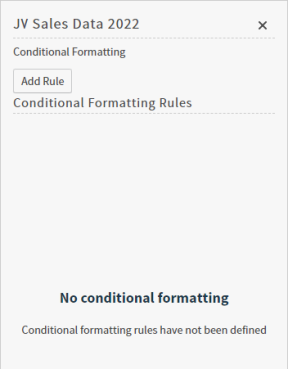
-
Using the Conditional Formatting sidebar, you can configure formatting options for your pivot table visuals. See Configure Conditional Formatting.
-
After making changes, select Apply to apply the conditional formatting rules you have specified.
-
Save the visual or dashboard to save your changes.
Conditional Format Options
The available options for rules and formatting change to reflect your selections.
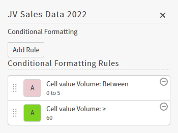
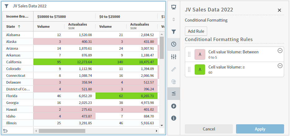
Conditional Formatting Sidebar
-
Select Add Rule to add a conditional formatting rule. See Configure Conditional Formatting.
-
Select an existing rule to edit the rule, or the delete icon (
 ) to delete the rule.
 -
Select and drag rules to change their order.
Add or Edit Conditional Formatting Rule
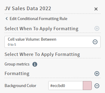
Select When To Apply Formatting
Select the add icon (![]() ) in Select When To Apply Formatting to define the conditions to apply your formatting.
) in Select When To Apply Formatting to define the conditions to apply your formatting.
Select Where To Apply Formatting
Select the add icon (![]() ) for Formatting to define the formatting for your condition.
) for Formatting to define the formatting for your condition.
Select the delete icon (![]() ) to delete a formatting option.
) to delete a formatting option.
Select When To Apply Formatting
Group attribute: Select a group of data to define values for that aggregated data. Optionally, select the add icon (![]() ) to add a derived field or custom metric.
) to add a derived field or custom metric.
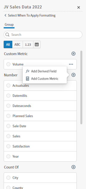
Example: Format Group attributes that meet the condition: the Range of Volume grouped by Income Bracket is Between a defined range of values.
Select Values for a Custom Metric
| Selection | Description |
|---|---|
| Values |
Select a range of values to format. Options include:
|
| Operator | Select an operator to use. Options may include Between, Equal, Not Equal, Greater Than, Greater Than or Equal, Less Than, and Less than or Equal. Depending on the Operator you select, different definition fields are available to use |
| From, To | Define a value range for Between. |
| Value | Define a value for Equal, Not Equal, Greater Than, Greater Than or Equal, Less Than, and Less than or Equal. |
Select Values for a Number
| Selection | Description |
|---|---|
| Range | Displays the range for this value. |
| Values |
Select a range of values to format. Options include:
|
| Aggregation | Select an aggregation option for Values. Options include Avg, Min, Max, Sum, Count, Distinct Count, and Last Value. |
| Operator | Select an operator to use. Options may include Between, Equal, Not Equal, Greater Than, Greater Than or Equal, Less Than, and Less than or Equal. Depending on the Operator you select, different definition fields are available to use. |
| From, To | Define a value range for Between. |
| Value | Define a value for Equal, Not Equal, Greater Than, Greater Than or Equal, Less Than, and Less than or Equal. |
Select Values for Count Of
| Selection | Description |
|---|---|
| Values |
Select a range of values to format. Options include:
|
| Aggregation | Select an aggregation option for Values. Options include Countand Distinct Count. |
| Operator | Select an operator to use. Options may include Between, Equal, Not Equal, Greater Than, Greater Than or Equal, Less Than, and Less than or Equal. Depending on the Operator you select, different definition fields are available to use. |
| From, To | Define a value range for Between. |
| Value | Define a value for Equal, Not Equal, Greater Than, Greater Than or Equal, Less Than, and Less than or Equal. |
Formatting
Select the add icon (![]() ) to add a formatting option you'll apply to your condition. Select the delete icon (
) to add a formatting option you'll apply to your condition. Select the delete icon (![]() ) to remove the formatting option.
) to remove the formatting option.
| Format Option | Description |
|---|---|
| Text Color | Select to define the text color format to apply to your condition. Enter the color number in hexadecimal, or use the color picker to enter RGB values or pick your color visually. |
| Background Color | Select to define the background color to apply to your condition. Enter the color number in hexadecimal, or use the color picker to enter RGB values or pick your color visually. |
| Bold | Select to enable or disable bold formatting to apply to your condition. |
| Italic | Select to enable or disable italic formatting to apply to your condition. |
| Underline | Select to enable or disable underline formatting to apply to your condition. |
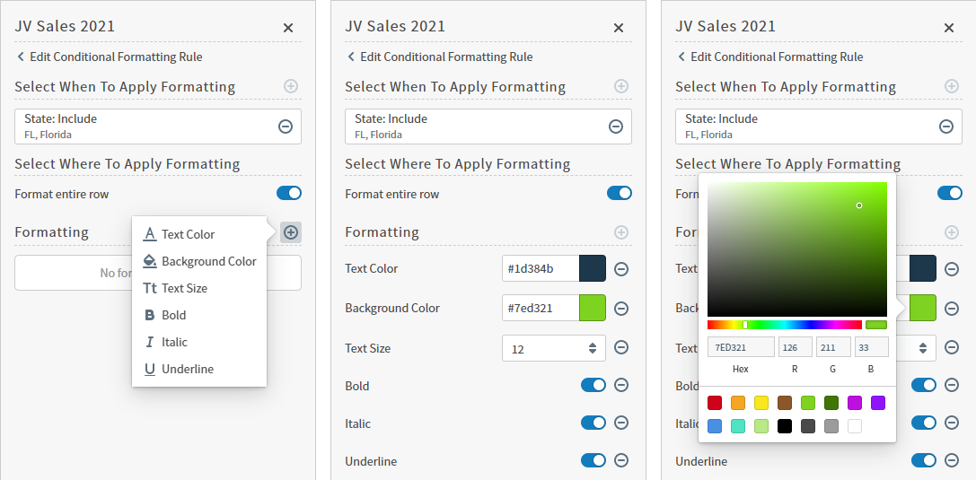
In the above example, formatting based on the Actualsales condition is applied first, then formatting based on the State condition overrides that rule.
Mix and match rules as needed to achieve the look and feel you want.